Comparing $z$ and $\chi^2$ tests

Mon 19 February 2018
Stats
#hypothesis, #testing, #z-test, #chi2-test

This post is a snapshot of a notebook that can be found here: (fd870a6). You can also enjoy the binder version of this notebook

import pandas as pd
import numpy as np
from scipy import stats
from statsmodels.stats import proportion

from ipywidgets import interact, interactive, fixed, interact_manual
import ipywidgets as widgets

%matplotlib inline
import seaborn as sns
import matplotlib.pyplot as plt
plt.style.use('ggplot')

Preface

The motivation for this tutorial is to better understand the methods to assess the results of A/B(/C...) tests. There are so many common pitfalls when it comes to A/B tests; make sure you avoid them! For example, this check list might be a good reference.

A common and repeating question is how to check the significance of the results of an A/B test. Matt Brems provided a very nice summary. I wanted to compare two of the tests suggested:

The plan

Let us define $N$ to be a set of $u$ integers and $\Delta$ to be a set of $v$ real numbers. For each $n \in N$ and $\delta \in \Delta$ we generate a synthetic results of an A/B test. In particular the control and variant groups would have $\sim n$ observations. The reason is that in real results of A/B tests, the groups sizes are normally not identical; they are close but not equal. Furthermore, the control set would have a fixed $\mathrm{CTR}$ (click through rate) and the variant will have conversion rate of $\mathrm{CTR} + \delta$.

As the null hypothesis we take that the CTR of the control and variant groups is the same, independently of the treatment. Thus a small $p$-value should suggest to reject the null hypothesis. For each synthetic result we will compute the $p$-value using a $z$-test and a $\chi^2$-test. In general, we expect that the smaller $n$ is and the larger $\delta$, the resulting $p$-value would be larger.

Generate data

Groups' sizes

In reality, even though we assume the users are split randomly and evenly, the final groups' sizes are not identical. Therefore, we randomize the group size:

def rand_group_size(N, tol=0.05):
    return N + np.random.randint(
        min(-tol * N, -1),
        max(tol * N, 1) + 1)

Event's value

For each successful event we assign a value. To that end we use a truncated uniform distribution providing the low and up values, together with the mean (mu) and standard deviation (sigma).

def rand_values(low, up, mu, sigma, N):
    return stats.truncnorm(
        (low - mu) / sigma,
        (up  - mu) / sigma,
        loc=mu, scale=sigma).rvs(N)

Generating the data for a group

When generating an observation, the following features are randomized:

The group size; controlled by N (~size) and N_tol. See rand_group_size
Name of the group. Normally control or var. Configured by treat.
Randomly assign 1 is the event was converted and 0 otherwise. The randomness is controlled by the weightctr
In case of conversion what was the value; controlled by: min_val, max_val, mean_val and std_val
What day of the test is it; controlled by number of days and the distribution days_dist
seed can help you reproduce the results.

def generate_group_observations(N=1000, N_tol=0.05,
                                treat='control',
                                ctr=0.2,
                                min_val=None, max_val=None,
                                mean_val=None, std_val=None,
                                days=7, days_dist=[1/7] * 7,
                                verbose=True,
                                seed=42
                               ):
    if verbose:
        print('Generating ~{N} samples with tolerance {tol}'.format(N=N, tol=N_tol))
        print('CTR: {ctr}'.format(ctr=ctr))
        print('Min value: {min_val} / Max value: {max_val}'.format(min_val=min_val,
                                                                   max_val=max_val))
        print('Value mean: {mean_val} / Value STD: {std_val}'.format(mean_val=mean_val,
                                                                     std_val=std_val))
        print('Generating observation over {days} days with {dist} as the distribution'.format(
            days=days, dist=days_dist
        ))
    if seed is not None:
        np.random.seed(seed)
    N = rand_group_size(N=N, tol=N_tol)
    converts = np.random.choice([0, 1], size=N, p=[1 - ctr, ctr])
    values = np.multiply(rand_values(min_val, max_val, mean_val, std_val, N), converts)
    day = np.random.choice(np.arange(0, days), p=days_dist, size=N)
    return pd.DataFrame(
        {
            "Treat": [treat] * N,
            "Day": day,
            "Converted": converts,
            "Value": values
        }
    )

Here is an example of ~10 observation (for a single group) spread along two days

generate_group_observations(
    N=10, days=2, days_dist=[0.4, 0.6],
    min_val=30, max_val=100, mean_val=60, std_val=20, seed=314)

Generating ~10 samples with tolerance 0.05
CTR: 0.2
Min value: 30 / Max value: 100
Value mean: 60 / Value STD: 20
Generating observation over 2 days with [0.4, 0.6] as the distribution

	Converted	Day	Treat	Value
0	1	1	control	58.682799
1	0	1	control	0.000000
2	1	1	control	83.425302
3	0	0	control	0.000000
4	1	0	control	37.115954
5	1	0	control	85.991153
6	0	1	control	0.000000
7	0	1	control	0.000000
8	1	1	control	53.225721

We are now ready to generate a synthetic results set of an A/B test, using the following function.

def generate_observations(N=1000,
                          control_ctr=0.2,
                          control_min_value=50,
                          control_max_value=150,
                          control_mean_sale=80,
                          control_std_sale=20,
                          var_ctr=0.15,
                          var_min_value=50,
                          var_max_value=150,
                          var_mean_sale=90,
                          var_std_sale=30,
                          days=7, days_dist=[1/7] * 7,
                          seed=42,
                          verbose=True
                         ):
    np.random.seed(seed)
    control = generate_group_observations(N=N, days=days, days_dist=days_dist,
                                          ctr=control_ctr, min_val=control_min_value, max_val=control_max_value,
                                          mean_val=control_mean_sale, std_val=control_std_sale,
                                          treat='control',
                                          seed=None, verbose=verbose
                                         )
    var = generate_group_observations(N=N, days=days, days_dist=days_dist,
                                      ctr=var_ctr, min_val=var_min_value, max_val=var_max_value,
                                      mean_val=var_mean_sale, std_val=var_std_sale,
                                      treat='var',
                                      seed=None, verbose=verbose
                                     )

    results = pd.concat([control, var]).reset_index(drop=True)
    return results

Here's a ~10 days X 2 (for control and variation groups) results set

generate_observations(N=10, seed=262, verbose=False)

	Converted	Day	Treat	Value
0	0	1	control	0.000000
1	1	6	control	90.575667
2	0	2	control	0.000000
3	0	0	control	0.000000
4	0	3	control	0.000000
5	0	6	control	0.000000
6	0	3	control	0.000000
7	1	5	control	88.962021
8	0	2	control	0.000000
9	0	3	control	0.000000
10	0	6	var	0.000000
11	0	6	var	0.000000
12	1	6	var	61.830611
13	0	2	var	0.000000
14	0	1	var	0.000000
15	0	6	var	0.000000
16	0	6	var	0.000000
17	1	4	var	74.639051
18	0	0	var	0.000000

Conversion rate

At this point we want to aggregate the results and compute the metric (a.k.a. proportion) we are after. In this example we consider the conversion rate.

def agg_conversion(results):
    conversions = results.groupby('Treat')['Converted'].agg(['count', 'sum'])
    conversions.rename(columns={'count': 'Visitors', 'sum': 'Converted'}, inplace=True)
    conversions['Not_converted'] = conversions.Visitors - conversions.Converted
    conversions['CR'] = conversions.Converted / conversions.Visitors
    return conversions

For the conversion rate we aggregate the raw events into a contingency matrix. Here is the resulting aggregation of the data generated previously.

agg_conversion(generate_observations(N=10, seed=262, verbose=False))

	Visitors	Converted	Not_converted	CR
Treat
control	10	2	8	0.200000
var	9	2	7	0.222222

Conversion rate and sample size

In this example (you have to run the notebook interactively) you can witness how the smaller the sample size is the further off the conversion rate is from the one prescribed in the generation function.

Fix the conversion rate for the control and variation groups
Play around with $N$. Note that the larger $N$ is the aggregation of the results gets closers to the values set.

For every value of $N$ we generate a synthetic data set and aggregate it to get the observed conversion rate. The synthetic

interact(
    lambda N, control_ctr, var_ctr: print(
        agg_conversion(
            generate_observations(
                seed=None, verbose=False,
                N=N,
                control_ctr=control_ctr,
                var_ctr=var_ctr
            ))['CR']
        ),
    control_ctr=widgets.FloatSlider(value=0.2, min=0, max=1, step=0.05, description='Control CR'),
    var_ctr=widgets.FloatSlider(value=0.15, min=0, max=1, step=0.05, description='Variation CR'),
    N=widgets.IntSlider(min=10,max=5000,step=100,value=1000)
);

Failed to display Jupyter Widget of type interactive.

If you're reading this message in the Jupyter Notebook or JupyterLab Notebook, it may mean that the widgets JavaScript is still loading. If this message persists, it likely means that the widgets JavaScript library is either not installed or not enabled. See the Jupyter Widgets Documentation for setup instructions.

If you're reading this message in another frontend (for example, a static rendering on GitHub or NBViewer), it may mean that your frontend doesn't currently support widgets.

Experimenting with different statistical tests

First, here is a simple utility to plot a heat map of the the resulting $p$-values.

def plot_experiment(df):
    """
    Utility function to plot a heatmap of the resulting p-values
    """
    plt.figure(figsize=(10,10))
    ax = sns.heatmap(df, cmap=plt.cm.Blues, linecolor='gray',
                     xticklabels=df.columns.values.round(2),
                     linewidths=.02
                    )
    ax.set(xlabel='CR delta', ylabel='N')
    ax.set_yticklabels(rotation=0, labels=Ns);

As discussed in the outline, we generate results for various $n$'s and various CTRs of the variant group.

def generate_data(control_ctr, deltas, Ns, seeds_seed=None):
    """
    Generate data for len(Ns)*len(deltas) experiment.
    Each experiment has ~N observation in each group and
    the CTR of the variation is control_ctr+delta
    """
    if seeds_seed is not None:
        np.random.seed(seeds_seed)
    seeds = np.random.randint(0, 2**32 - 1, size=(len(Ns), len(deltas)))
    experiments = [
        [
            generate_observations(
                N=N, control_ctr=control_ctr,
                var_ctr = control_ctr + delta,
                seed=seeds[i][j] if seeds_seed is not None else None,
                verbose=False
            ) for j, delta in enumerate(deltas)
        ] for i, N in enumerate(Ns)
    ]
    return pd.DataFrame(experiments, index=Ns, columns=deltas)

Finally, generating the data:

deltas = np.linspace(-0.15, 0.15, num=31)
Ns = np.round(np.linspace(10, 10000, num=40)).astype('int64')

data = generate_data(seeds_seed=262, control_ctr=0.2,
                     deltas=deltas, Ns=Ns,
                    )

For each A/B test we aggregate the data:

data_agg = data.applymap(agg_conversion)

Utility function to element-wise $p$-value computation:

def compute_proportions_pvals(data_agg, test):
    """
    Compute the p-value of a single A/B test.
    `test` is assumed to be from `statsmodels.stats.proportion`
    """
    return data_agg.applymap(lambda x: test(x['Converted'], x['Visitors'])[1])

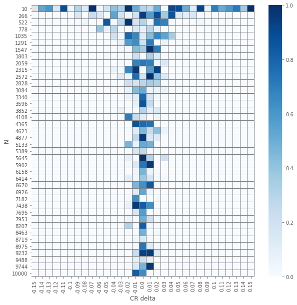
$\chi^2$ independence test

pvals_chi2 = compute_proportions_pvals(data_agg, proportion.proportions_chisquare)
plot_experiment(pvals_chi2)

/Users/drorata/anaconda3/envs/z-vs-ch2-tests/lib/python3.6/site-packages/scipy/stats/stats.py:4554: RuntimeWarning: invalid value encountered in true_divide
  terms = (f_obs - f_exp)**2 / f_exp

png

$z$ test

pvals_z = compute_proportions_pvals(data_agg, proportion.proportions_ztest)
plot_experiment(pvals_z)

/Users/drorata/anaconda3/envs/z-vs-ch2-tests/lib/python3.6/site-packages/statsmodels/stats/weightstats.py:670: RuntimeWarning: invalid value encountered in double_scalars
  zstat = value / std_diff

png

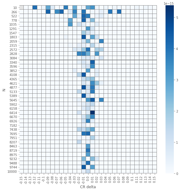
Comparing $z$-test and $\chi^2$ test

The results of the element-wise $z$ and $\chi^2$ tests yields an expected visualization. The smaller the number of samples per group $N$ is and the smaller $\delat$ is we have $p$-values that are larger. But, and it is not a huge surprise, the visuals for the two different tests seems similar. Let us check how close are they.

pvals_diffs_close = pd.DataFrame(np.isclose(pvals_chi2, pvals_z))

pvals_diffs = (pvals_chi2 - pvals_z).abs()

plot_experiment(pvals_diffs)

png

plot_experiment(pvals_diffs_close.applymap(lambda x: 0 if x else 1))

png

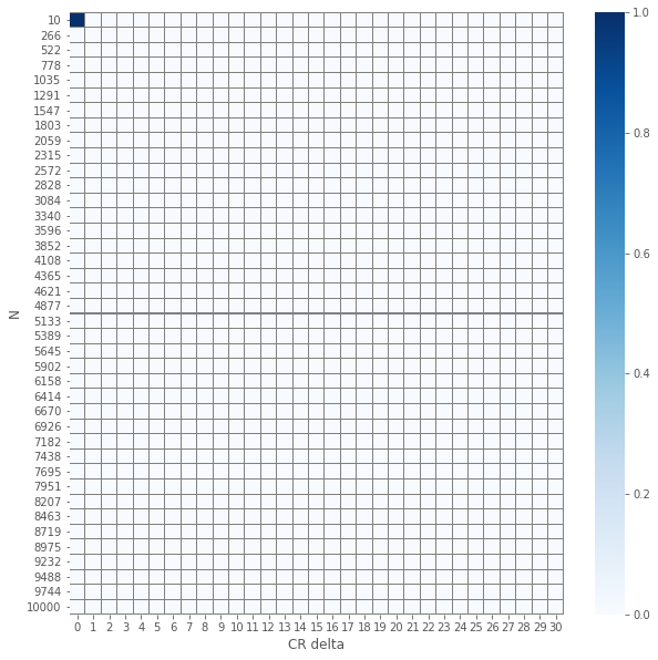
So we see that except a single(!) case, all $p$-values are the same!

Dr. Dror